How to outperform the Bitcoin Market using a self-developed Deep Reinforcement Learning Trading Bot

Key Takeaways

I developed my own Bitcoin Deep Reinforcement Learning Trading Bot
Price, volume, trade related and market indicators are used
A feedforward neural network is trained using trade data from 2015-2018
The bot decides every day, if it should hold Bitcoin or not
After 15 months of live trading, the bot outperforms a buy & hold approach significantly

Overview

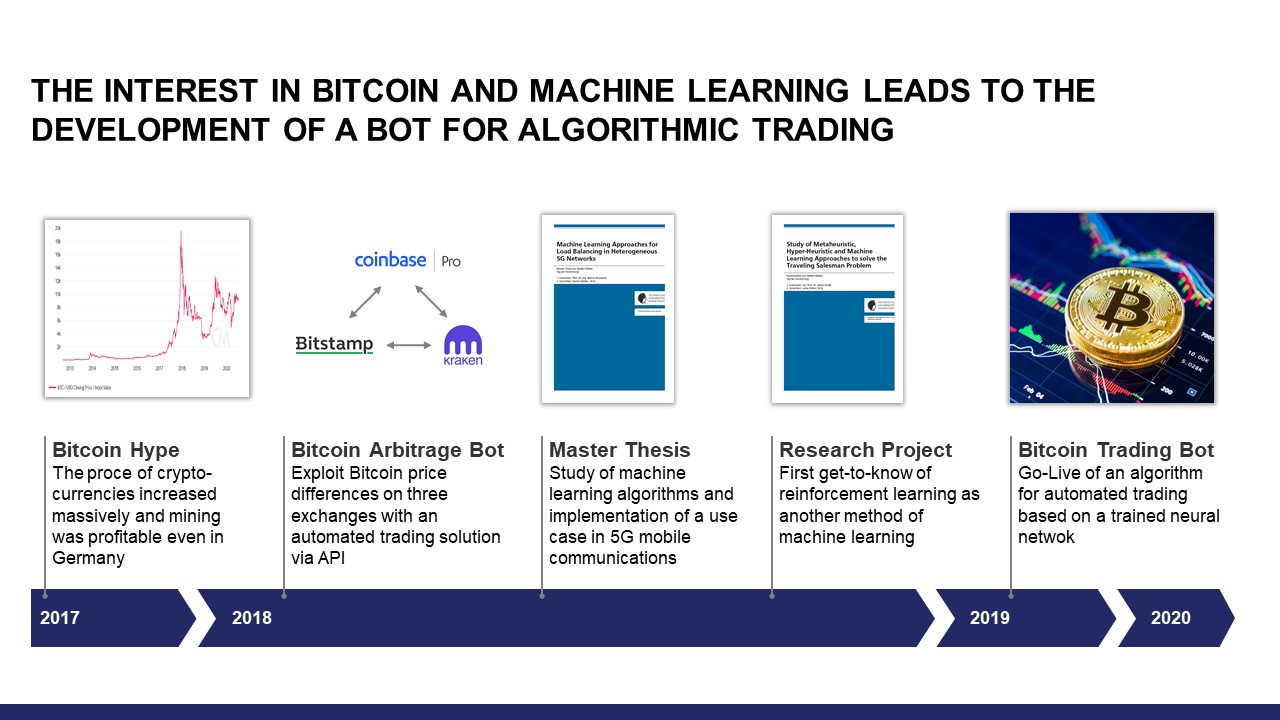
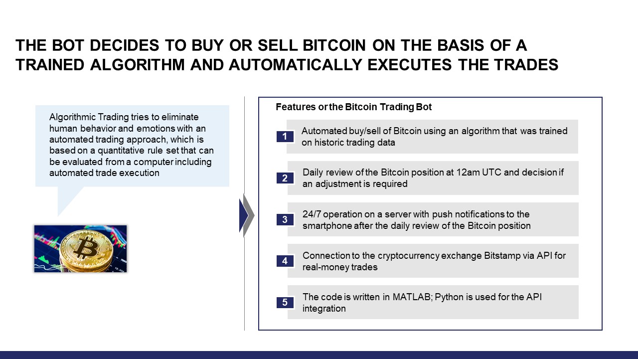
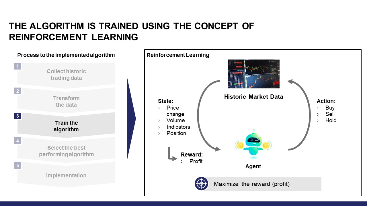
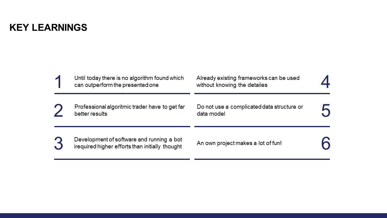
For an overview of the Bitcoin trading bot please have a look at this presentation or the following slides. For non-technical readers I recommend to skip chapter 3 of this article.

1. Introduction and motivation

Do you invest in Bitcoin? Have you ever heard about algorithmic trading and the possibility to earn money with it or to outperform the market? In this article, these two topics come together. I will tell you my story about developing and running a Bitcoin trading bot. This includes the results after over one year of live trading with real money. It all starts in the beginning of 2018…

In the beginning of 2018, I worked on my master’s thesis in communication technology. The goal was to evaluate different machine learning approaches to assign users to cellular network base stations in a smart way to lower the highest load factor of any base station in the system. Using the optimal allocation of users to base stations, a supervised machine learning algorithm (e.g. Support Vector Machine) was trained to predict the best base station for a given user.
During these times, I thought of developing a Bitcoin trading bot. However, training a supervised machine learning algorithm requires training data with in this example successful trades. At this point, I did not know how to obtain this data and so I did not follow the idea any longer..
Instead, I developed an arbitrage bot that executes trades automatically if there are any significant differences in Bitcoin price between certain fiat exchanges. The description of this arbitrage bot might follow in another article.

In mid 2018, I worked on a research project with the goal to introduce approaches to solve the well-known Traveling Salesman Problem (TSP). For example, there exist many meta-heuristics to solve the TSP. In addition, the TSP can be solved with reinforcement learning as I described in my research project:

“Reinforcement learning is learning what to do in order to maximize a numerical reward signal. The learner is not told which actions to take, but instead must discover which actions yield the most reward by trying them. Often, actions affect not only the immediate reward but also the next situation and all subsequent rewards. These two characteristics, trial-and-error and delayed reward, are the main features of reinforcement learning.
In contrast to supervised learning, a reinforcement learner does not learn from labeled training sets. For this reason, reinforcement learning can be applied to most combinatorial optimization problems, because supervised learning is not applicable due to the fact that one does not have access to optimal labels. For example, an agent could learn to play a game by being told whether it wins or loses, but is never given the “correct” action at any given point in time. For this reason, a reinforcement learning approach is used to approximate the best tour for the TSP.”

If you want to know more about reinforcement learning, have a look at my research project, which includes many references to articles about solution approaches for the TSP.

While writing the reinforcement learning part of the research project, I realized that this approach solves the problem of unknown labels when using a supervised learning approach. That is why I searched the web for reinforcement learning approaches for Bitcoin to know more about this concept. There were many interesting approaches and some are linked below:

The inspiration to develop a reinforcement learning trading bot by myself was triggered by article [1] in combination with the description in article [5] of how to implement deep learning algorithms. It has to be noted that most of the research was done in late 2018. Maybe some good articles about Bitcoin trading bots have been released in the meantime.

After finishing my research project in August 2018, I started developing first concepts for the trading bot. If you are interested in more details, please let me know and send me an email. In the next chapter, the prerequisites to be able to train and run the bot are presented.

2. Prerequisites

Obtain data

To train an algorithm, we need lots of historical trade data. The fiat currency pair with the highest liquidity is BTC/USD and so I looked for the best available data in this trading pair. Bitstamp is one of the oldest exchanges, but there is no way to pull historical data from their official API. That is why I chose Coinbase Pro (GDAX) for historical trade data. Using their API, I downloaded every single trade since the beginning of 2015. In addition to price and volume information of a trade, an indication is available that shows if the trade results of a sell or buy side order. An example for the information provided for one trade is shown below:

Table 1: Trade information for each trade using the Coinbase Pro API.

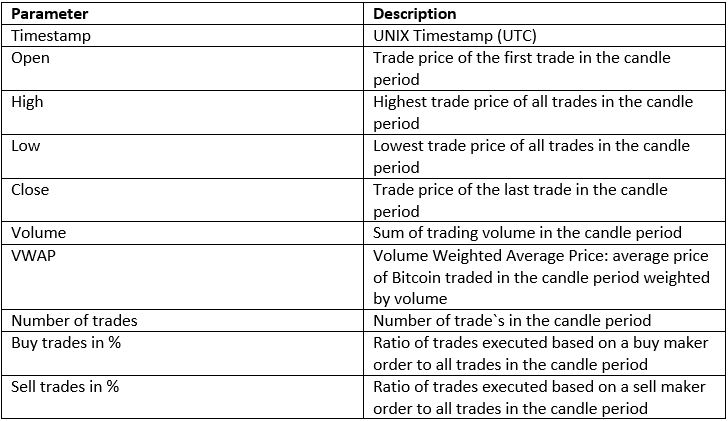
In the next step, all trades (in sum about 90 millions in May 2020) are transformed into candlesticks or OHLC (Open-High-Low-Close) for different time periods. Common periods in trading are 5m, 15m, 30m, 1h, 4h, 12h and 24h. The additional sell/buy side indication is transformed into a percentage value which reflects the ratio of sell/buy trades to all trades in this candle.
Calculating the data from all trades reveals the problem of missing trade data for a few days. This is due to downtimes of the exchange, sometimes for several days in a row. To obtain a continuous series of candles, historical pre-calculated candles from Bitstamp are used, which I found on Kaggle. In sum, the following parameters are available for each candle period:

Table 2: Calculated values for each candle stick period.

Market indicators

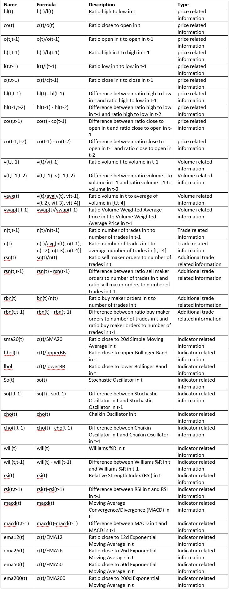
With candlesticks, volume and additional trade information available one can calculate different market indicators. There exist many indicators, but I wanted to stick to the ones that get attention from traders. Especially, article [4] inspired my selection of market indicators.
In addition to these indicators, the algorithm has to know about recent price action. This information is included using the relative price action in the last periods. However, this kind of information can lead to overfitting. Therefore, I only used simple types of relations between parameters in different periods.
In the following, I will call market indicators and additional information just “indicators”. All used indicators are shown in the table below:

Table 3: All used indicators to train the bot.

I also evaluated other indicators like the volatility, which is commonly used in stock trading. For example, the VXX measures the volatility of the S&P 500 and is used as some kind of market sentiment indicator (very high = panic). Unfortunately, using different timeframes for the volatility in addition to the presented indicators, the performance of the bot do not change. That is why I excluded volatility as an indicator. However, the relative price action in comparison to the 5-days-average price is some kind of implicit volatility.

In addition to indicators, data transformations can be used to improve the training data for the learning algorithm. In article [1], they used the so-called z-score transformation. It transforms the data into mean and standard deviation in order to compare values of different scale or values which increase/decrease over the time. I applied this approach, but the results were worse than before. However, there was one learning for me. Values have to be comparable and on the same scale over time, which means that you should use relative values instead of differences between raw values. Then, the algorithm can learn the general relationship between parameters. For example, the number of trades is an integer value and maybe it will increase over the time, because more people are interested in trading Bitcoin. If the absolute number of trades is used as an input for training, the algorithm can predict an incorrect state when this number changes. This can easily happen in case of an event, which has nothing to do with the overall market situation. That is why most of the price and trade indicators are measured in percent.

Obtaining training data for the algorithm requires the calculation of the indicators for each candlestick. In sum, one has to calculate 37 indicator values for each candlestick period. Using this series of indicator values, we are ready to train the algorithm. In the next chapter, the key concepts and technical descriptions of the bot are presented

3. Model

Concept of Reinforcement Learning

As described before, using the concept of reinforcement learning I trained an algorithm or a so-called policy. In the following, an excerpt of my research project about solving the TSP is presented to explain Markov Decision Processes, which is a mathematical representation of reinforcement learning.

The formal problem of finite Markov Decision Processes (MDPs) involves evaluative feedback and choosing different actions in different situations. MDPs are a classical formalization of sequential decision making, where actions influence not just immediate rewards, but also subsequent situations or states. These future rewards can be seen as delayed reward from an action. MDPs involve delayed reward and the need to trade-off immediate and delayed reward. Regarding the TSP, immediate reward is a short path to the next city and delayed reward is the overall tour length. A large immediate reward may lead to a sub-optimal result. For this reason, learning has to be applied to choose the optimal trade-off value. In MDPs, learning is achieved by interaction with the environment to reach a goal. The learner and decision maker is called agent. It interacts with everything outside itself which is called environment. Both interact continually, the agent selecting actions and the environment responding to these actions and presenting new situations or states to the agent. In addition, the environment gives rise to rewards, which are special numerical values that the agent wants to maximize over time through its choice of actions.

Agent States and Actions

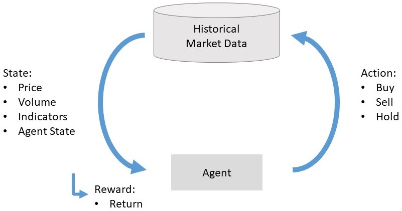
In our case, the agent can choose between three states as shown in the following table:

If the predicted agent state differs from the actual state, this will result in an action of the agent to change to the new state. The interaction of agent and environment is illustrated in Fig. 1.

Figure 1: Interaction of agent and environment.

I also evaluated other states, where the agent can short Bitcoin. However, the performance during bull markets is worse and that is why I used the presented states.

Episodes

In order to let the agent explore the solution space, the complete time series is split into subsequences, which are called episodes. These episodes are a fragment of the whole time series. One reason to do this is to handle the complexity of the problem. Including many states and a long time series, the optimization problem grows exponentially. In my case, I chose an episode length of 96 candles. Why 96? Initially, this length was chosen to reflect that one episode is equal to one day when using 15m candlesticks. I never changed this, because in my opinion it is a good trade-off between the complexity and length of the timeframe.

Q-Learning

As I started learning more about the implementation of reinforcement learning, I tried to understand the concept of Q-learning, where an agent optimizes one episode and the result is used as input for a supervised learning algorithm. However, the agent has to explore the solution space with in my case 3⁹⁶ solutions (=6×10⁴⁵), which is a really large number, and would require lots of computation effort. Reducing the number of candles in each episode might result in other problems and so I decided to follow the second approach for reinforcement learning and trained the policy directly.

Train the Policy directly

Article [1] helped me a lot to understand the concept of learning a policy directly. In this case, the agent plays an episode based on the prediction of the most promising state for the future given by the policy (e.g. a neural network).
In learning mode, a randomization factor is introduced to reflect the process of learning and is called learning rate. In my case, I choose a learning rate of 10%. This means that in learning mode the agent takes a random state in 10% of each decisions. If the random decision leads to a good result (=reward) of an episode, then the policy will be optimized in such a way that this is reflected. If the random decision leads to a bad result of an episode, the performance of the policy will mostly not be affected. This is because when playing an episode, the agent takes the state with the highest predicted value for the maximum return. Using this scheme, the agent will explore the solution space and the policy is constantly improved.

The Policy

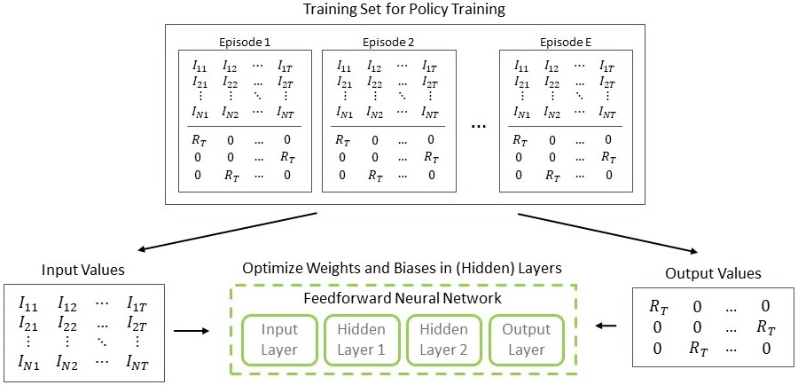
The policy used for the trading bot is a neural net with 40 inputs and 3 outputs. The inputs are the indicators and a representation of the last state. The output is the expected reward at the end of an episode for each possible state. I use a simple feedforward neural net with two hidden layers as policy.
One goal of this project is to keep it simple and to do not overfit the algorithm using large neural nets with many hidden layers. Applying the rule of thumb for the size of each hidden layer, I defined the first layer to have 40 inputs according to the 40 input values and the second layer to have 30 inputs.

Figure 2: Used feedforward neural net with two hidden layers.

Training Algorithm Concept

In order to train the feedforward net, the agent plays random episodes. The data for each decision and the reward at the end of each episode is collected. Then, the reward is used as the output of the net for the state that the agent has chosen. If the reward is high, then the policy will be optimized in a way that it reflects this high reward in future decisions when the input is of the same pattern of indicators. Fig. 3 shows a high-level overview of the training process.

Figure 3: High-level overview of the training process.

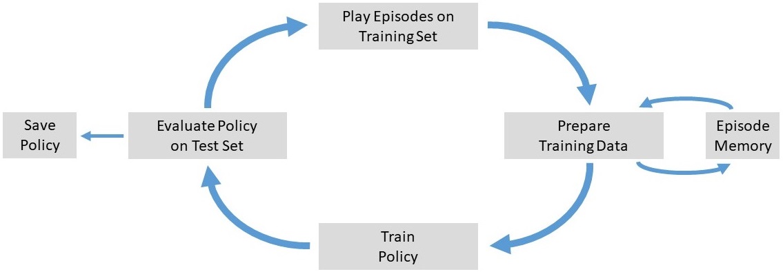
In the next Sections, the detailed concept of each phase is presented. If you want to skip these technical descriptions, you can jump to the description of selecting the best policy in Chapter 4.

Play Episodes on Training Set

In order to start training the policy, one has to collect training data as described in Chapter 2. In the next step, using the introduced learning rate of 10%, the agent explores the environment. For each input column vector there is a chance that the agent picks a random new state. If the agent chooses the policy, the state with the highest output becomes the new state. After calculating the series of states for an episode, the reward of the whole episode is calculated. This process is summarized in Fig. 4.

Figure 4: Playing episodes on the training set.

Prepare Training Data

As illustrated in Fig. 5, the collected episode data consisting of input indicators, output states and reward is transformed into training data to optimize the policy. In order to be able to train the policy, the state representation is replaced by the episode reward. Then, the obtained training data is saved in the episode memory, which contains all played episodes. Using additional episodes from the memory when training the policy can reduce the problem overfitting, because it introduces previous knowledge from other played episodes.

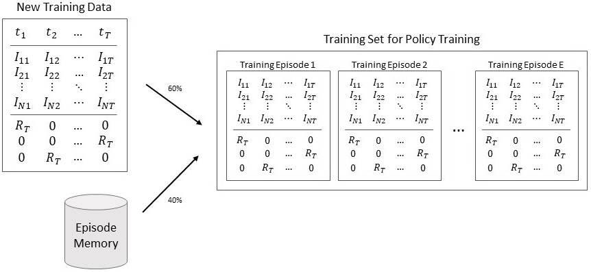
Figure 6: Prepare training data to optimize the policy using newly played episodes and episodes from the episode memory.

After 50 played episodes, the final training data to optimize the policy is prepared as shown in Fig. 6. Using a fraction of the data from newly played episodes and a fraction from the episode memory, the training set is ready to be used for training.

Train Policy

In this step, the last feedforward neural network is optimized based on the training set. The input and output values of the training set are known as illustrated in Fig. 7. Therefore, a backpropagation algorithm can be used to calculate the weights and biases of the neural network nodes and connections.

Figure 7: Optimizing the policy using the training set and a backpropagation algorithm.

Evaluate Policy on Test Set

Every 2,500 episodes, the policy is evaluated on the test set without any random learning factor. The data set consists of the whole data since 2015. Choosing the agent state with the highest predicted future reward each time leads to the series of agent states. Using this series, the reward of the whole time series since is calculated. Both, reward and policy are saved for manual comparison at a later stage. This process is illustrated in Fig. 8 shown below.

Figure 8: Evaluation of the policy on the whole data set.

Parameters for training

After finishing the code of the presented training algorithm, I started training the policy. There exist different parameters, which can be fine-tuned. For each combination of parameters, the reinforcement learning agent plays 150,000 episodes. The following Table 5 provides an overview of the used parameters for training.

After several code iterations and re-starts (bug fixing etc.), the final training started in December 2018. Performing the training simultaneously with one instance of training on each CPU core, it took 2 weeks to train in sum 30 different parameter combinations.

As described before, all trained policies are saved for manual comparison. In the next chapter, the comparison of different policies and the selection of one of them is described.

4. Selection of the best Policy

I started training the bot with candlesticks and indicators on lower time scales (e.g. 15m, 30m, 1h or 4h). The results were not bad, but including trading fees (even low fees with just 0.005%) would cause a massive loss and a bad performance. By design the bot is able to trade after each candle, if the prediction of the most promising state for the future changes. This can lead to a high trade frequency and that is why I decided to use only 12h and 24h candles for training.
Using 12h candles the bot can quickly react to market changes, but the problem with trading fees still apply. A real trading bot requires doing nothing when the market trades sideways. Therefore, I stick to daily candles and the goal of the bot is to outperform a buy & hold (HODL) approach over the long term. This is the origin of the nickname Deep Reinforcement Learning HODL Bot, which I gave the bot during development.

Training the algorithm with different parameter combinations on daily candles took a lot of time and effort. However, the selection of the best policy took even more time. In sum, training leads to about 1000 neural nets/policies. Each of these policies was evaluated on a data set with all data available to this point in time. In addition to the performance in percent compared to a buy & hold approach, other performance criteria are calculated as shown below.

Return compared to a buy & hold approach (in %)
Sharpe Ratio
Maximum drawdown
Trade frequency (since this is a buy & hold approach, one wants to pay as less trading fees as possible)

Evaluating the performance of each policy including these additional criteria is easier than only using the overall performance. Nevertheless, 100 out of the 1000 policies had to be evaluated manually to get an impression of the performance in different market phases. This is some kind of a soft factor and has a high impact on the decision which policy to use, because one gets a feeling for the behavior of the bot for different market situations.
After all the manual evaluation of policies, my key observations are as follows:

A larger training set leads not necessarily to a better policy
Using z-score values instead of normal values has no positive impact on the overall performance
Trading fees can eat your performance and that is why the trade frequency is an important number as an indicator for overall trading costs
Including trading fees in the training leads to worse results compared to training without fees (both evaluated including the trading fees)
Many policies outperform a buy & hold approach
The bot misses the start of a bullish market phase
During bull markets, the bot slightly underperforms a buy & hold approach
At the beginning of a bear market / market crash, the bot mostly finds a good selling point
During bear markets, the bot outperforms a buy & hold approach

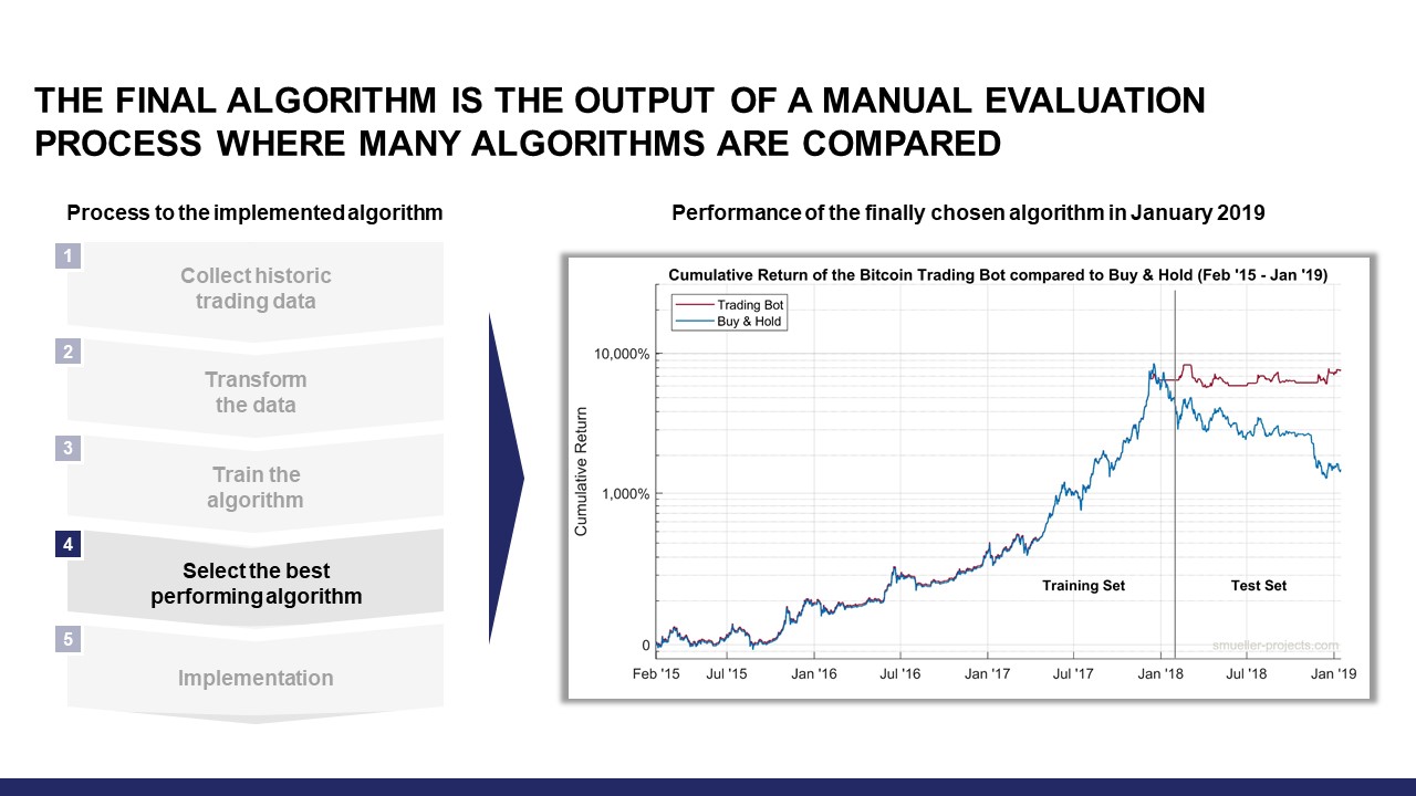
Now the question is: which policy did I choose in January 2019 and how did it perform since then?
I chose a policy that was trained on a training set including all candles from January 2015 to February 2018. Despite the small training set compared to the available data until January 2019, the performance during the bear market since February 2018 was impressive and a buy & hold approach was easily outperformed.
In addition, the policy always found a good selling point before downward movements. This observation was one of the key criteria to choose this policy. If the policy acts like this in unknown market situations during the last bear market, I can expect that it will prevent me from massive losses in future bear markets.
The numeric results including charts and all performance measures are presented in Chapter 6. Before that, the implementation of the bot is described in the next Chapter 5.

5. Implementation of the Bot

The bot is written in MATLAB using parts of the Machine Learning Toolbox and some additional Python scripts to connect to the exchange. The market data is collected 24/7 on my own server. For the daily close and the calculation of the daily candle, I decided to take 0 UTC as the best time. In BTC markets, there is no real market close each day and that is why many people stick to 0 UTC (including charting websites like TradingView).

As described before, the bot decides which Bitcoin position it wants to hold every 24 hours (0%, 50% or 100% of the investment capital used). Using real money, the bot executes trades on Bitstamp. The trades are executed in the BTC/EUR pair, but the trading decision is based on the BTC/USD pair. Therefore, fluctuations in the EUR/USD pair can lead to a different trading performance compared to a USD-only based trading. However, all charts in this article and on the website are based on the BTC/USD pair.
Each day after 0 UTC, predicted futures rewards of each possible state and possible trade execution results are documented. In addition, every day I receive a push notification on my mobile phone using Pushbullet with a summary report. In future, I might switch to Pushover as notification app, because for a one-time purchase one can receive far more push notifications each month (7500 instead of 100).

In the next Chapter 6, the performance results including 15 months of live trading are presented.

6. Trading Performance

After all the descriptions of the bot and the technical details, there is one question left. How is the performance of the bot? Does it outperform the market and a buy & hold approach? Let us have a look at the results.

January 2015 – January 2019

Back in January 2019, I chose a policy that was optimized using trading data that excludes the last 350 days. Therefore, the training set included three years of data from the beginning of 2015 to the beginning of 2018. The performance of this policy compared to a buy & hold approach and evaluated in January 2019 is shown below in Fig. 9. Because of the large increase of Bitcoin price, a logarithmic chart is used.

Figure 9: Performance of the bot compared to a buy & hold at the time I decided to use this policy for live trading.

This was the overall best policy out of hundreds of policies. I chose this one, because of the low drawdown and “selling at the top” in the beginning of 2018. If this policy outperforms a buy & hold approach during bear markets in a way that it do not hold any Bitcoin for a long time, this is completely fine for me. In addition, this policy executed a very small amount of trades in 3 years. This behavior can save a lot of trading fees as described before.

January 2015 – May 2020

Looking at the performance of the bot 15 months later, it still outperforms the market and a buy & hold approach as illustrated in Fig 10. The overall performance is really impressive with about a 250x of return compared to January 2015 while the price of Bitcoin only increased only about 45x. In addition, let us remember that the policy was trained using data until January 2018 and since then, the bot is running without any further training.

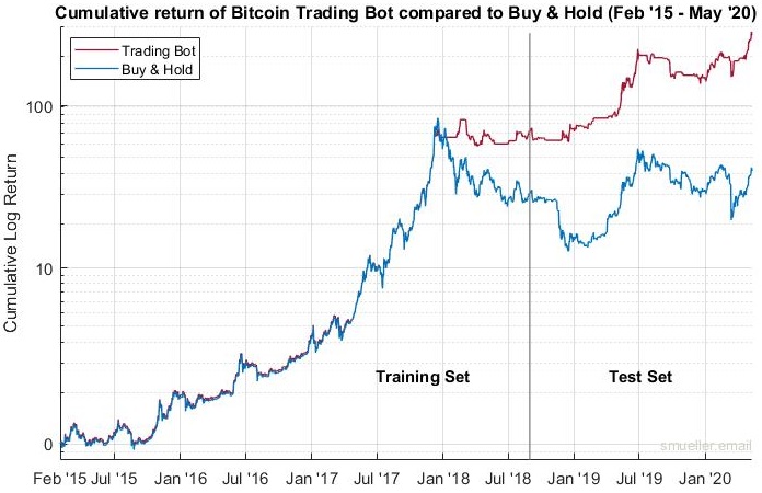
Figure 10: Performance of the bot compared to a buy & hold from January 2015 – May 2019.

Due to the logarithmic chart, it is hard to recognize the performance differences of the bot and the buy & hold approach in the last 15 months. Therefore, let us have a closer look at the live trading timeframe.

January 2019 – May 2020

The performance of the trading bot in the last 15 months is shown in Fig. 11.

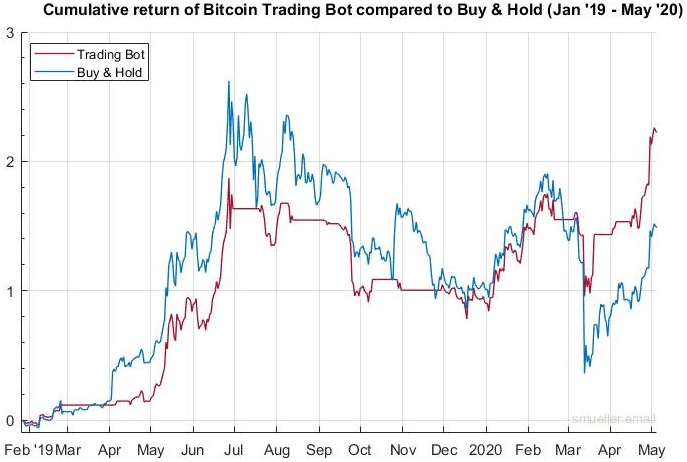
Figure 11: Performance of the bot compared to a buy & hold in the 15 months of live trading.

During these months, the bot traded 34 times, but missed to enter the market in April 2019 when the overall sentiment turned bullish. Due to this, the performance lagged behind the market for a few weeks. However, the bot was able to catch up on March 12th 2020, when the Bitcoin price dropped by nearly 50%, probably due to the selloff in the stock market. One day before that event, the bot changed its state to 1 which resulted in selling 50% of the Bitcoin holdings. Maybe this was just luck, but I evaluated other policies, which were trained using candlesticks data until February 2020, and they show the same behavior of selling half or all of their holdings before that price drop.
In sum, the bot is now outperforming the market with 48 percentage points or 30 percent. The detailed numbers and performance measures are shown in Table 6.

Table 6: Performance measures of the Deep Reinforcement Learning Trading Bot compared to a buy & hold approach, January ’19 – May ‘20.

In addition to the charts presented in this chapter, you can have a look at the live trading results of my bot on the charts page. The chart is updated every day after the bot makes the decision to stick to its current state or to change the state.

7. Conclusion

When someone would have told me in August 2018 how much effort and work this project would require, there would be a high chance that I would have never started this project. Nevertheless, when I look back at hundreds of hours of researching, coding, evaluating and implementing, it have the feeling that it was the right decision to start this project. I learned a lot about coding in MATLAB/Python, APIs, data analysis, running code 24/7, Bitcoin markets and much more. It is great to see all these articles about algorithmic trading and Bitcoin, because now I can state that it works! Many thanks to all authors that inspired me for this project.

If you have any questions, just send me an email. Thank you for reading!
-Steffen

Disclaimer: This article is no financial advice. Furthermore, I am an engineer and apply frameworks to reach a certain goal without knowing the deep technical characteristics. Therefore, the given explanations can include mistakes. If you find one, please let me know.